Petri Nets

Petri nets are a powerful way to model discrete event systems - systems where events happen one step at a time. They’re used to visualize how events unfold, interact, and depend on each other. Because of this, they’re also known as place/transition nets or simply P/T nets.

Where does the name come from?

Petri nets are named after their inventor, the German computer scientist Karl Adam Petri, who developed the idea back in the 1960s.

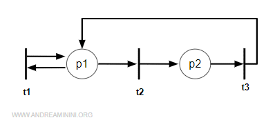
Here’s a simple, visual example of what a Petri net looks like:

Note. In most cases, a Petri net is a logical model of a discrete event system (DES) that doesn’t include time as a factor. However, there are also versions called timed Petri nets that do. The place/transition net is just the simplest and most common kind.

How a Petri Net Works

A place/transition Petri net (P/T net) is defined by two sets and two matrices:

$$ N = \{ P, T, Pre, Post \} $$

In simple terms, you can picture it as a directed graph - that is, a diagram made of circles and rectangles connected by arrows, where each arrow can carry a numerical weight.

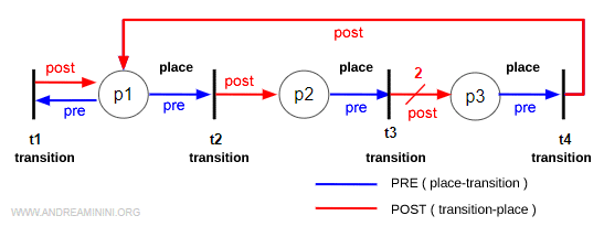
Places (p) are shown as circles. They represent the system’s states or conditions. Formally, the set of all places is written as:

$$ P = \{ p_1, p_2, p_3, ... \} $$

Transitions (t) are shown as bars or rectangles. They represent the events that can change those states. The set of transitions is written as:

$$ T = \{ t_1, t_2, t_3, ... \} $$

Note. Both places and transitions are nodes in the graph. They’re drawn differently so you can easily tell them apart. By definition, the two sets are disjoint - they don’t share any elements: P⋂T=ø.

Arrows connecting places to transitions are called pre-incidence arcs and are stored in a matrix called Pre(p,t).

It’s called “Pre” because it counts how many input arcs go into each transition.

Arrows connecting transitions to places are called post-incidence arcs and are stored in another matrix, Post(p,t).

It’s called “Post” because it counts the number of output arcs that leave each transition.

 

Note. In both matrices, places are listed in rows and transitions in columns. Each cell contains a non-negative integer that shows whether an arc exists (1) or not (0). If the number is greater than 1, it means there are multiple arcs between those two nodes.

Often, these two matrices - Pre and Post - are combined into a single, compact form called the incidence matrix:

$$ C = Post - Pre = \begin{pmatrix} 1-1 & 0-1 & 0 & 1 \\ 0 & 1 & 0-1 & 0-1 \\ 0 & 0 & 2 & 0-1 \end{pmatrix} = \begin{pmatrix} 0 & -1 & 0 & 1 \\ 0 & 1 & -1 & -1 \\ 0 & 0 & 2 & -1 \end{pmatrix} $$

Each element in the incidence matrix represents the algebraic difference between the corresponding elements in the Post and Pre matrices:

$$ C(p,t) = Post(p,t) - Pre(p,t) $$

Note. This format simplifies things, but it does lose some information. For instance, if a place and a transition are connected by the same number of reciprocal arcs (forming a loop), their difference will still be zero - as if no connection existed. So, even if loops are actually there, the net appears as a pure (loop-free) one.

Each element in the net is connected to other elements through incoming and outgoing links.

By convention, an asterisk before the element (*n) indicates incoming links, while placing it after (n*) shows outgoing ones.

Example. Place p₁ has the following connections: incoming *p₁ = {t₁, t₄} and outgoing p₁* = {t₁, t₂}. The same applies to transitions. Transition t₁ has incoming links *t₁ = {p₁} and outgoing ones t₁* = {p₁}.

A Practical Example

Let’s explore how a Petri net actually works by building a simple example step by step. Our net has three places:

$$ P = \{ p_1, p_2, p_3 \} $$

and four transitions:

$$ T = \{ t_1, t_2, t_3, t_4 \} $$

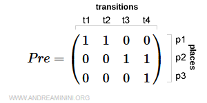
The pre-incidence matrix (places → transitions) shows how many input arcs lead into each transition:

$$ Pre = \begin{pmatrix} 1 & 1 & 0 & 0 \\ 0 & 0 & 1 & 0 \\ 0 & 0 & 0 & 1 \end{pmatrix} $$

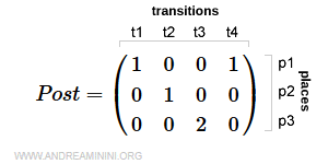
The post-incidence matrix (transitions → places) does the opposite - it shows how many output arcs leave each transition:

$$ Post = \begin{pmatrix} 1 & 0 & 0 & 1 \\ 0 & 1 & 0 & 0 \\ 0 & 0 & 2 & 0 \end{pmatrix} $$

To draw the corresponding digraph, we represent each place P with a circle and each transition T with a bar or rectangle:

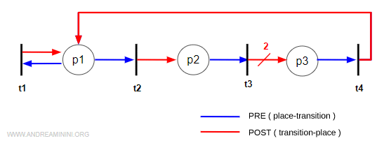
Then we connect them using directed arcs according to the Pre and Post matrices:

• For every positive value in the Pre matrix, draw a red arc from the place to the transition.
• For every positive value in the Post matrix, draw a blue arc from the transition to the place.

Note. A zero in the matrix simply means there’s no arc. A positive integer indicates one or more arcs. If the value n is greater than 1, it means there are n arcs connecting those nodes. Instead of drawing all of them, it’s cleaner to draw one arc and label it with the number of arcs - for example, the connection between t₃ and p₃ represents two arcs. This makes the graph much easier to read at a glance.

The Marked Net

Now let’s add one more layer: a marking, which represents the current state of the Petri net.

A marking assigns a non-negative integer to each place, showing how many tokens it contains at a given moment. In other words, it describes what’s happening in the system right now.

The markings are collected in a vector M, with one value for each place:

$$ M = \{ m_1, m_2, m_3, ... \} $$

Visually, tokens are drawn as small black dots placed inside the circles (the places):

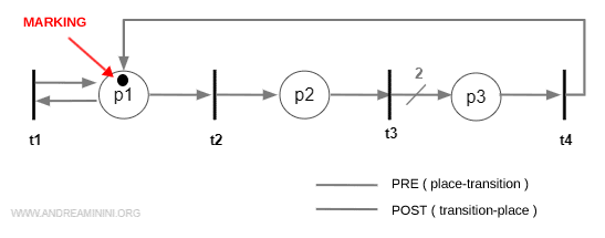
Here’s a quick example:

This marking vector assigns one token to p₂, two tokens to p₄, and none to the other places:

$$ M = \{ 0, 1, 0, 2 \} $$

The Marked Petri Net

A marked Petri net (or net system) is a place/transition net that starts with an initial marking M₀ defining its initial state: $$ <N, M_0> $$

This initial configuration determines how the system behaves and evolves over time. Each firing of a transition changes the marking, leading to a new state of the net - and that’s how Petri nets model the flow of events in dynamic systems.

Why Petri Nets Matter

So, why are Petri nets such a valuable tool? Here are some of the key reasons:

• They’re compact yet expressive. Petri nets pack a lot of information into a clean, visual structure that makes it easier to understand how a system behaves.

  Example. A Petri net doesn’t list every possible state - instead, it defines the rules of how the system changes. This makes it possible to represent systems with infinitely many states, something that traditional finite automata can’t do efficiently.

• They bridge visuals and math. A Petri net isn’t just a diagram - it’s also a formal mathematical model. That means you can analyze it using linear algebra to explore its properties, such as reachability or invariants.
• They’re modular by design. You can model each subsystem separately as its own module (or sub-net) and then connect them - just like building blocks.
• They naturally represent concurrency. Petri nets are perfect for systems where several activities happen at once - for example, in distributed computing, workflow management, or manufacturing processes.

In short, Petri nets offer a unique blend of clarity and analytical power, making them an essential tool for anyone studying or designing complex dynamic systems.