Simple Linear Regression
Simple linear regression is a statistical model that describes the relationship between two numerical variables. It’s one of the most commonly used techniques in both descriptive and inferential statistics.
The model assumes that the dependent variable $Y$ can be expressed as a linear function of the independent variable $X$, plus a random error term.
In mathematical form:
$$ Y = a + bX + \varepsilon $$
Where:
- $Y$ is the response (dependent) variable
- $X$ is the predictor (independent) variable
- $a$ is the intercept
- $b$ is the slope (regression coefficient)
- $\varepsilon$ is the random error term (unobserved)
The intercept $a$ represents the expected value of $Y$ when $X = 0$. It’s the point where the estimated regression line crosses the vertical axis.
The slope $b$ indicates the average change in $Y$ for every one-unit increase in $X$. It represents the marginal rate of change.
How do we estimate $ a $ and $ b $?
At the outset, the values of $a$ and $b$ are unknown. They’re estimated from sample data using the least squares method.
This approach finds the coefficients $\hat{a}$ and $\hat{b}$ by minimizing the sum of squared differences between the observed values $y_i$ and the predicted values $\hat{y}_i$:
$$ \text{SSE} = \sum_{i=1}^n (y_i - \hat{y}_i)^2 $$
The estimation formulas are:
$$
\hat{b} = \frac{ \sum (x_i - \bar{x})(y_i - \bar{y}) }{ \sum (x_i - \bar{x})^2 }
\quad ; \quad
\hat{a} = \bar{y} - \hat{b} \bar{x}
$$
A practical example
Suppose we want to predict test scores based on weekly study hours.
Let’s say the data analysis yields:
$$ \hat{a} = 50 \quad ; \quad \hat{b} = 2 $$
The estimated regression equation is:
$$ \hat{y} = 50 + 2x $$
If a student doesn’t study at all ($x = 0$), the expected score is 50.
Each additional hour of study per week is associated with an expected increase of 2 points.
Note. This model does not deliver exact predictions-it estimates an expected average based on the available data.
Example 2
Consider a small sample of 5 observations recording:
- $ X$: number of study hours
- $Y$: preparation level (measured on a 0-100 scale)
The dataset is as follows:
| i | xi (hours) | yi (score) |
|---|---|---|
| 1 | 1 | 55 |
| 2 | 2 | 58 |
| 3 | 3 | 60 |
| 4 | 4 | 63 |
| 5 | 5 | 65 |
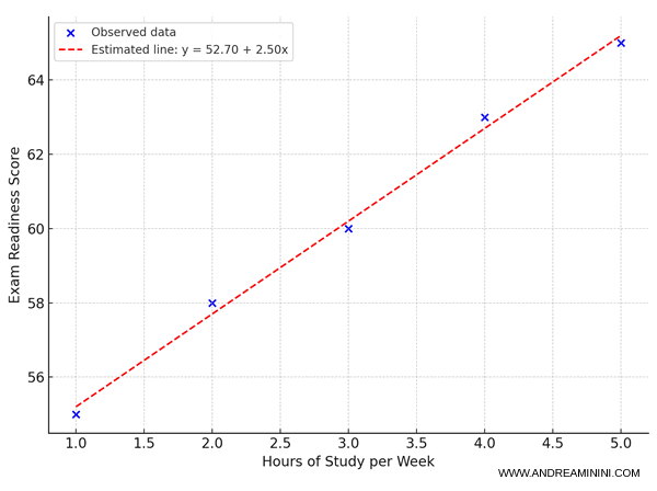
We want to estimate the regression line $\hat{y} = \hat{a} + \hat{b}x$, but neither the slope nor the intercept is known yet.
Step one is to compute the sample means:
$$ \bar{x} = \frac{1 + 2 + 3 + 4 + 5}{5} = \frac{15}{5} = 3 $$
$$ \bar{y} = \frac{55 + 58 + 60 + 63 + 65}{5} = \frac{301}{5} = 60.2 $$
Next, calculate the numerator for $\hat{b}$, namely $\sum (x_i - \bar{x})(y_i - \bar{y})$:
| i | \(x_i - \bar{x}\) | \(y_i - \bar{y}\) | Product |
|---|---|---|---|
| 1 | \(1 - 3 = -2\) | \(55 - 60.2 = -5.2\) | \((-2)(-5.2) = 10.4\) |
| 2 | \(2 - 3 = -1\) | \(58 - 60.2 = -2.2\) | \((-1)(-2.2) = 2.2\) |
| 3 | \(3 - 3 = 0\) | \(60 - 60.2 = -0.2\) | \(0 \cdot (-0.2) = 0\) |
| 4 | \(4 - 3 = +1\) | \(63 - 60.2 = 2.8\) | \(1 \cdot 2.8 = 2.8\) |
| 5 | \(5 - 3 = +2\) | \(65 - 60.2 = 4.8\) | \(2 \cdot 4.8 = 9.6\) |
Summing these products gives:
$$ 10.4 + 2.2 + 0 + 2.8 + 9.6 = 25.0 $$
Now, compute the denominator for $\hat{b}$, i.e., $\sum (x_i - \bar{x})^2$:
| i | \(x_i - \bar{x}\) | Square |
|---|---|---|
| 1 | \(-2\) | 4 |
| 2 | \(-1\) | 1 |
| 3 | 0 | 0 |
| 4 | \(+1\) | 1 |
| 5 | \(+2\) | 4 |
The sum of squares is:
$$ 4 + 1 + 0 + 1 + 4 = 10 $$
We can now estimate the slope $\hat{b}$:
$$ \hat{b} = \frac{25.0}{10} = 2.5 $$
and the intercept $\hat{a}$:
$$ \hat{a} = \bar{y} - \hat{b}\,\bar{x} = 60.2 - 2.5 \cdot 3 = 60.2 - 7.5 = 52.7 $$
The estimated regression line is therefore:
$$ \hat{y} = 52.7 + 2.5x $$
Interpretation: if a student does not study ($x = 0$), the predicted score is $\hat{y} = 52.7$.
On average, each additional study hour per week is associated with a 2.5-point increase in the score.

At this stage, we can also compute the residuals $e_i = y_i - \hat{y}_i$ for each observation to assess model fit. For example:
- For $i = 1$: $\hat{y}_1 = 52.7 + 2.5 \cdot 1 = 55.2$. Residual $e_1 = 55 - 55.2 = -0.2$.
- For $i = 2$: $\hat{y}_2 = 52.7 + 2.5 \cdot 2 = 57.7$. Residual $e_2 = 58 - 57.7 = 0.3$.
- And so forth.
If the residuals are “small” and show no clear pattern, the model can be considered adequate. But if they exhibit systematic behavior (for instance, consistently increasing with $x$), one or more assumptions are likely being violated.
Model limitations
The model rests on several assumptions:
- Linearity: the relationship between $X$ and $Y$ is straight-line.
- Homoscedasticity: the variance of the errors is constant.
- Independence of errors.
- Normality of errors (for inference).
If one or more of these assumptions are violated, the model may no longer be appropriate.
For example, if the relationship between $X$ and $Y$ is curved, a straight line will fail to capture the pattern accurately.
This is why applying simple linear regression always requires an empirical check of model adequacy. It’s often the first step before moving on to more advanced statistical frameworks.
Although basic, simple linear regression provides the foundation for more sophisticated statistical methods and paves the way for both theoretical and applied developments.
What are possible extensions of the model?
One major extension is multiple regression, which generalizes the simple linear model to include more than one independent variable.
In this case, the dependent variable is explained not by a single factor but by a set of predictors.
This makes it possible to describe more realistic scenarios, where multiple, interconnected influences come into play.
Another important extension involves nonlinear models.
When the relationship between the variables is not linear, a straight line is no longer adequate. In such cases, more flexible functions-such as quadratics, logarithmic curves, or exponential functions-are used to better fit the observed data.
Simple regression also introduces several key concepts, such as:
- The coefficient of determination $R^2$, which measures how much of the variability in $Y$ is explained by the model. A value close to 1 indicates strong explanatory power, while a low value suggests the model fails to capture the underlying structure.
- Residual analysis, which examines the differences between observed and predicted values. This analysis is crucial for detecting anomalies, evaluating goodness-of-fit, and checking whether the statistical assumptions hold.
In short, despite its simplicity, this model is an essential starting point for anyone aiming to build solid proficiency in statistical analysis.

