Concurrent Composition of Petri Nets
Given two labeled Petri nets N1 and N2, the concurrent composition of the resulting net N3 is obtained by merging the transitions that share the same label. $$ L(N_3)= L(N_1)||L(N_2) \\ L_m(N_3)= L_m(N_1)||L_m(N_2) $$
Concurrent composition makes it possible to synchronize two modules by pairing up their transitions whenever they carry the same label. When this happens, the transitions are merged into a single composite transition that fires only if it is enabled in both modules. In practice, this mechanism ensures that the synchronized transitions occur at the same time, allowing the two systems to evolve in step with each other.
Nota. Concurrent composition is not limited to two transitions. It can be applied to any number of synchronous transitions that share the same label.
A practical example
Consider two labeled Petri nets, G1 and G2:
$$ G_1 = (N_1, l_1, m_{0,1}, F_1 ) $$
$$ G_2 = (N_2, l_2, m_{0,2}, F_2 ) $$
The diagrams below show the structure of the two modules.
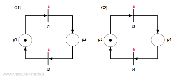
Each module uses a labeling function to associate symbols with its transitions. In our example, the first module has:
$$ l_1 (t_1) = a \\ l_1 (t_2) = a $$
while the second module has:
$$ l_2 (t_3) = a \\ l_2 (t_4) = b $$
The sets of final markings are:
$$ F_1 = \{ [1 \: 0] \} $$
$$ F_2 = \{ [1 \: 0], [0 \:1] \} $$
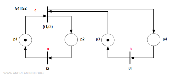
We can now combine the two modules through concurrent composition:
$$ G = G_1 || G_2 $$
Since transitions t1, t2, and t3 all share the label “a”, they are considered synchronous and may be merged into a single transition. This is illustrated below.
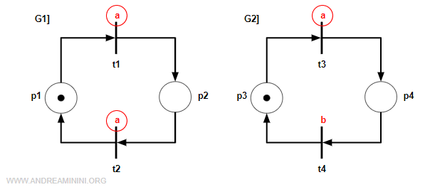
Nota. Only the pairs t1 - t3 and t2 - t3 belong to different modules. Even though t1 and t2 share the same label, they are part of the same module. In cases like this, when multiple transitions inside a module have the same label, they must each be paired with the matching transitions in the other module. This produces the two combinations t1 - t3 and t2 - t3.
We now merge the transitions step by step. First, we combine t1 and t3, creating the composite transition (t1,t3):
Next, we merge t2 and t3, obtaining the composite transition (t2,t3):
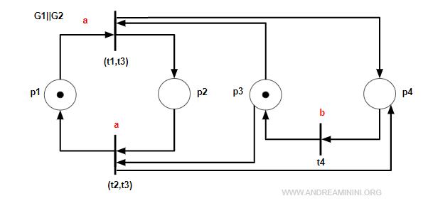
The initial marking of the composed net is:
$$ m_0 = [1 \: 0 \: 1 \: 0] $$
Nota. Each position in the vector represents a place in the composed net. Since the marking contains one token in p1 and one in p3, the resulting marking is [1 0 1 0].
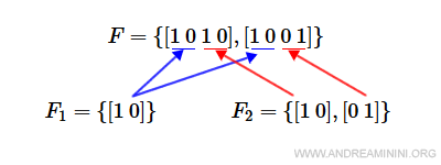
The final states of the composed net are all the combinations of F1 and F2:
$$ F = \{ [1 \: 0 \: 1 \: 0] , [1 \: 0 \: 0 \: 1] \} $$
Nota. The first two positions of each vector remain the same because they correspond to F1=[1,0]. The last two positions differ, since F2 includes both [1,0] and [0,1].
The complexity of concurrent composition
The Petri net that results from concurrent composition contains the union of the places from both modules:
$$ |P|=|P_1|+|P_2| $$
The transitions, however, depend on how many labels are shared between the modules. If no labels are repeated within each module, then the number of transitions satisfies:
$$ |T| \le |T_1|+|T_2| $$
More generally, combining k modules yields:
$$ n = k \cdot (|T_1|+|T_2|) $$
This means that the overall complexity of the composed Petri net grows linearly with the number of modules. This is a major advantage because it prevents the rapid growth of the state space that often affects composed systems.
Nota. In many systems, the state space grows exponentially as more components are added. Petri nets help avoid this by keeping the structure manageable.
However, if a module contains repeated labels assigned to multiple transitions, the construction becomes more complex and requires additional care.